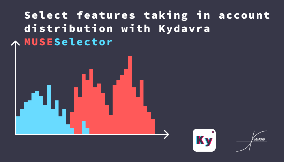
One of the most intuitive ways to select features would be to find how much the distribution of the classes is different from each other. However on some intervals, the distribution of the feature by the classes can be different, but on other intervals, it can be practically the same. So, we can deduce that the features that have the most intervals where the distribution of classes differ are the best features. This logic is implemented in Minimum Uncertainty and Sample Elimination (or shortly MUSE) implemented in kydavra as MUSESelector.

Using MUSESelector from Kydavra library.

If you still haven’t installed Kydavra just type the following in the following in the command line.

pip install kydavra

If you already have installed the first version of kydavra, please upgrade it by running the following command.

pip install --upgrade kydavra

Next, we need to import the model, create the selector, and apply it to our data:

from kydavra import MUSESelector

muse = MUSESelector(num_features = 5)
selected_cols = muse.select(df, 'target')

The select function takes as parameters the panda’s data frame and the name of the target column. The MUSESelector takes the following parameters:

• num_features (int, default = 5) : The number of features to retain in the data frame.
• n_bins (int, default = 20) : The number of bins to split data in for numerical features.
• p (float, default = 0.2) : The minimal value for the cumulated sum of probabilities of positive class frequency.
• T (float, default = 0.1) : The minimal threshold of the class impurity for a bin to be passed to the selector.

We strongly recommend you to experiment only with the num_features parameter and let the others with the default settings.

Let’s see an example:

Now we are going to test the performance of the MUSESelector on the heart disease UCI data set.

The default cross_val_score is.

0.8239

After applying the standard settings of the model the cross_val_score of the selected columns is.

0.6983164983164983

Not so good. However we can find a better result by trying more values for num_features.

from kydavra import MUSESelector
acc = []
for i in range(1, len(df.columns)-1):
    muse = MUSESelector(num_features=i)
    cols = muse.select(df, 'target')
    X = df[cols].values
    y = df['target'].values
    acc.append(np.mean(cross_val_score(logit, X, y)))

The result is the following:

[0.5475420875420876,
 0.5991245791245792,
 0.6027609427609428,
 0.691043771043771,
 0.6983164983164983,
 0.6948148148148148,
 0.7428956228956229,
 0.7792592592592593,
 0.804915824915825,
 0.8123905723905723,
 0.8345454545454546,
 0.8233670033670034]

We can see that by eliminating one column we can get more accuracy.

BONUS:

We can get even more accuracy by applying PCAFilter on the data. Check out how to use it. The result is:

1 - 0.801952861952862
2 - 0.7945454545454546
3 - 0.8092255892255892
4 - 0.8383164983164983
5 - 0.841952861952862
6 - 0.8274074074074076
7 - 0.8236363636363636
8 - 0.8200673400673402
9 - 0.8200673400673402
10 - 0.8274074074074076
11 - 0.842087542087542
12 - 0.8311111111111111

Again we can see that with the 11 features the cross_val_score is higher than the base model.

If you used or tried Kydavra we highly invite you to fill this form and share your experience.

Made with ❤ by Sigmoid.

Resource:

• https://drive.google.com/file/d/1G2eJyyL63xwRkyw_GBBthpyH7sD96N87/view?usp=sharing

Discussion